Why Instance Diversity Matters in Quantum Computing Research
Most quantum algorithm benchmarks test on a narrow set of problem instances. Regular graphs, uniform weights, shallow circuits. The result? We end up with algorithms that look great on paper but break down in practice. This post explains why instance diversity matters, and how Instance Space Analysis helps us understand when and why the Quantum Approximate Optimisation Algorithm (QAOA) actually works.
This work forms part of Chapters 3 and 4 of my PhD thesis, supervised by Prof. Kate Smith-Miles and Prof. Lloyd Hollenberg at the University of Melbourne.
Why Quantum Computing?
Quantum computers can theoretically solve some problems much faster than classical computers. Shor's algorithm for factoring large numbers could break RSA encryption. Grover's search offers a quadratic speedup over classical search. And quantum simulation promises breakthroughs in chemistry and materials science.
But there's a catch. The hardware is hard. Assuming no errors we need several thousands of qubits, and with current error rates, we'd need millions of qubits plus hundreds of millions of gates. We're currently in the NISQ era (Noisy Intermediate-Scale Quantum), with devices of 50 to 100 qubits that are noisy and error-prone.
The key idea is superposition: quantum bits (qubits) can exist in a superposition of states. A qubit state is represented by a vector in a complex vector space $|\psi\rangle \in [\mathbb{C}^2]^{\otimes n}$. For $N=300$ qubits, there are $2^{300}$ possible states, more than the number of atoms in the universe.
This has led to the development of Variational Quantum Algorithms (VQAs), hybrid classical-quantum algorithms specifically designed for NISQ devices. The focus here is on one prominent example: the Quantum Approximate Optimisation Algorithm (QAOA).
The MaxCut Problem
QAOA is a low-depth algorithm designed to solve optimisation problems. Many problems can be mapped to a Hamiltonian and solved using QAOA (e.g. MaxCut, TSP, Vehicle Routing, 3SAT). We use MaxCut as the testbed: partition a graph $G = (V, E)$ into two sets $S$ and $V \setminus S$ such that the number of edges between them is maximised:
$$\max_{\mathbf{s}} \sum_{(i,j) \in E} w_{ij} (1 - z_i z_j)$$
where $z_i \in \{0, 1\}$ and $w_{ij} \in \mathbb{R}$ is the weight of edge $(i, j)$. The solution is a binary string $\mathbf{s} = (s_1, s_2, \ldots, s_n)$ and the optimal objective value is $C_{\max}$.
To solve this on a quantum computer, we map it to a Hamiltonian. The classical objective becomes a quantum operator:
$$H = \sum_{(i,j) \in E} w_{ij} (I - Z_i Z_j)$$
where the state space moves from $\mathbf{s} \in \{0, 1\}^n$ to $|\psi\rangle \in \mathcal{H}_2^{\otimes n}$, and the solution becomes the ground state $|\psi_{\text{ground}}\rangle = \arg\min_{|\psi\rangle} \langle \psi | H | \psi \rangle$.
How QAOA Works
QAOA prepares a parameterised "trial" (ansatz) state of the form:
$$|\psi(\vec{\gamma}, \vec{\beta})\rangle = \prod_{j=1}^{p} e^{-i\beta_j \hat{H}_B} e^{-i\gamma_j \hat{H}_P} |+\rangle^{\otimes n}$$
where $\hat{H}_P = \sum_{(i,j) \in E} w_{ij} (1 - \hat{Z}_i \hat{Z}_j)$ is the problem Hamiltonian and $\hat{H}_B = \sum_{i=1}^{n} \hat{X}_i$ is the mixing Hamiltonian. The parameters $\vec{\gamma} = (\gamma_1, \dots, \gamma_p)$ and $\vec{\beta} = (\beta_1, \dots, \beta_p)$ are optimised to minimise the expectation value:
$$F_p(\vec{\gamma}, \vec{\beta}) = \langle +|^{\otimes n} \left(\prod_{j=1}^p e^{-i\beta_j \hat{H}_B} e^{-i\gamma_j \hat{H}_P}\right)^\dagger \hat{H}_P \left( \prod_{j=1}^{p} e^{-i\beta_j \hat{H}_B} e^{-i\gamma_j \hat{H}_P} \right) |+\rangle^{\otimes n} = \langle \psi(\vec{\gamma}, \vec{\beta}) | \hat{H}_P | \psi(\vec{\gamma}, \vec{\beta}) \rangle$$
The goal is to find optimal parameters $(\vec{\gamma}^*, \vec{\beta}^*) = \arg \min_{\vec{\gamma}, \vec{\beta}} F_p(\vec{\gamma}, \vec{\beta})$, and we measure solution quality via the approximation ratio $\alpha = F_p(\vec{\gamma}^*, \vec{\beta}^*) / C_{\max}$.
There are three key design decisions that significantly impact QAOA's performance:
- Circuit depth ($p$): controls the expressivity of the ansatz. As $p \rightarrow \infty$, QAOA can find the exact solution.
- Classical optimiser: gradient-free (Nelder-Mead, COBYLA) or gradient-based (ADAM, SPSA).
- Initial parameters ($\vec{\gamma}_0, \vec{\beta}_0$): various strategies for initialisation (TQA, INTERP, and our novel QIBPI approach).
The Problem: One Size Doesn't Fit All
Current QAOA research has significant limitations:
- Narrow focus on specific instance classes ($d$-regular graphs, random graphs, no weights)
- Predominantly shallow depth circuits ($p \leq 3$)
- Limited understanding of how instance features impact QAOA performance and design decisions
- Lack of standardised parameter initialisation frameworks
This led to three research questions:
- RQ1: How can we generate diverse MaxCut instances beyond current QAOA research?
- RQ2: How do instance characteristics influence key QAOA design decisions?
- RQ3: Can we develop methods to automatically optimise QAOA parameters based on instance features?
Instance Space Analysis
Instance Space Analysis (ISA), based on the No Free Lunch Theorem (that algorithms have strengths and weaknesses), provides a framework to understand when different algorithms perform well. Instead of reporting "on-average" performance, ISA identifies which algorithms are best suited for which instances by projecting them onto a 2D space.
The analysis requires four components of metadata $\{ \mathcal{I}, \mathcal{F}, \mathcal{A}, \mathcal{Y} \}$:
- Instances $\mathcal{I} \subseteq \mathcal{P}$: what instances show diversity of features
- Features $\mathcal{F}$: what features capture instance hardness
- Algorithms $\mathcal{A}$: what algorithm configurations show diversity
- Performance $y \in \mathcal{Y}$: how do we define performance
Our Instance Space
We analysed 4,200 MaxCut instances across 42 instance classes (7 network structures x 6 weight distributions), characterised by 48 features spanning structural, spectral, cycle-based, and weight-based properties.
Network structures included random, 3-regular, 4-regular, geometric, Watts-Strogatz, and nearly complete bipartite graphs. Weight distributions ranged from uniform and exponential to normal, gamma, and lognormal.
ISA projects the high-dimensional feature space onto 2D via a learned projection transformation matrix $\mathbf{Z}$:
$$\begin{pmatrix} z_1 \\ z_2 \end{pmatrix} = \begin{pmatrix} -0.52 & -0.59 & 0.40 & -0.14 & -0.01 & 0.42 & 0.08 & 0.00 & -0.20 & 0.34 \\ 0.23 & 0.74 & -0.26 & -0.20 & 0.51 & -0.02 & 0.65 & -0.09 & -0.35 & -0.38 \end{pmatrix} \begin{pmatrix} \text{algebraic connectivity} \\ \text{average distance} \\ \text{clique number} \\ \text{diameter} \\ \text{maximum degree} \\ \text{maximum weighted degree} \\ \text{number of edges} \\ \text{radius} \\ \text{skewness weight} \\ \text{weighted average clustering} \end{pmatrix}$$
This projects the 4,200 instances across $\mathbb{R}^2$, selecting 10 of the 48 features that best separate performance differences.
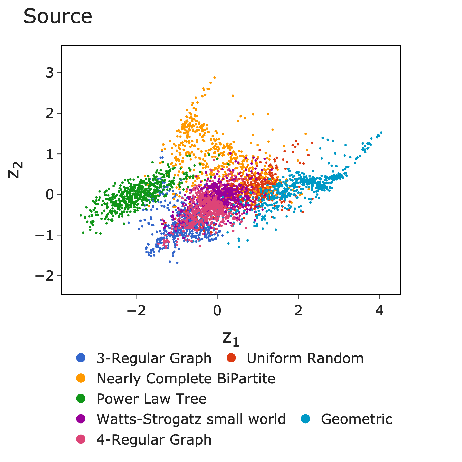
4,200 MaxCut instances projected onto 2D instance space, coloured by source class.
Performance Metric
Rather than just measuring approximation ratio $\alpha$, we defined performance as the number of function evaluations $\kappa$ needed to reach $\alpha_{\text{acceptable}} = 0.95 \cdot \alpha_{\max}$. If the algorithm never reaches this threshold, we assign a penalty $\kappa = 10^5$. This captures both solution quality and computational efficiency.
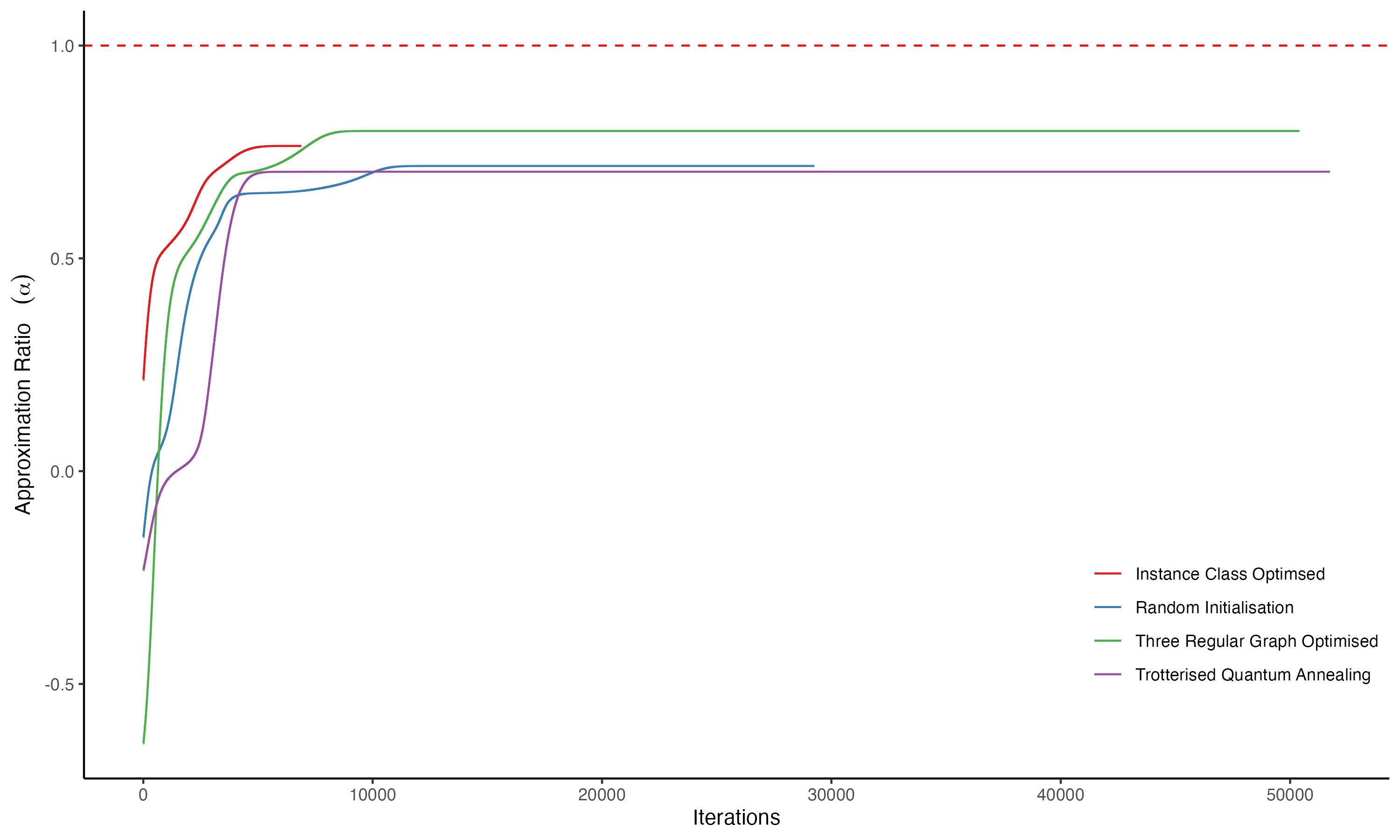
Approximation ratio for various instances across different initialisation techniques.
Three Independent Studies
We conducted three independent studies, each isolating one key design choice:
- IS I: Layer depth ($p \in \{2, 5, 10, 15, 20\}$). How many layers are needed for different instances?
- IS II: Classical optimiser selection (Nelder-Mead, Conjugate Gradient, Powell, SLSQP, L-BFGS-B). Which optimiser requires fewer calls to the quantum device?
- IS III/IV: Initialisation technique (Random, TQA, INTERP, Constant, QIBPI, Three-Regular). Can we achieve faster convergence to optimal parameters?
QAOA Landscape Complexity
The optimisation landscape of QAOA varies dramatically across instances. Higher circuit depth means more complex landscapes. Cauchy weight distributions produce more rugged landscapes. More complex landscapes require more calls to the QPU, and classical optimisers can falter, meaning more resource use.
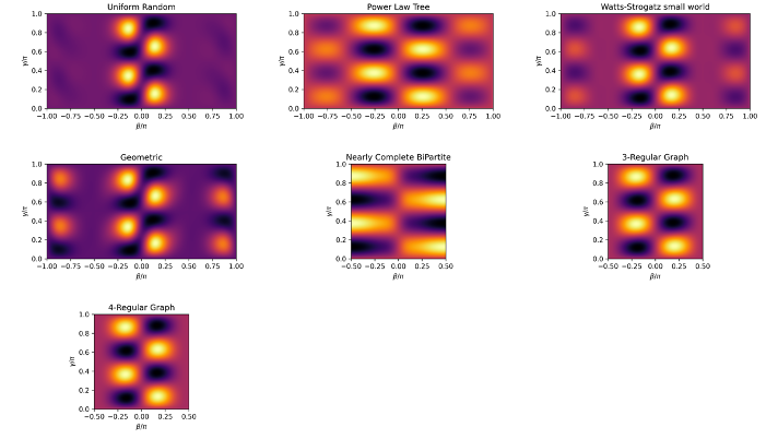
QAOA landscape variation across MaxCut instances (p=1, unweighted).
Key Results: Parameter Initialisation
The most impactful finding came from Instance Space III, studying parameter initialisation. We compared several strategies for setting initial parameters $(\vec{\gamma}_0, \vec{\beta}_0)$ at depth $p=15$:
Random: $\gamma_i \sim \mathcal{U}(-\pi, \pi)$, $\beta_i \sim \mathcal{U}(-\pi/2, \pi/2)$
TQA (Trotterized Quantum Annealing): $\gamma_i = i \cdot \Delta t / p$, $\beta_i = (1 - i/p) \cdot \Delta t$
CONSTANT: $\gamma_i = 0.2$, $\beta_i = -0.2$
FOURIER: $\gamma_i = \sum_k u_k \sin\!\left((k-\tfrac{1}{2})(i-\tfrac{1}{2})\tfrac{\pi}{p}\right)$
INTERP (Interpolation): $[\gamma_0^{(p+1)}]_i = \tfrac{i-1}{p} [\gamma_L^{(p)}]_{i-1}$
We developed QIBPI (Quantum Instance-based Parameter Initialisation), where pre-optimised parameters are derived from median values across 100 instances per class and depth level. For each of 42 graph types $T$ and each depth $p \in \{1, \ldots, 15\}$, we generate 100 instances, optimise QAOA with random initialisation, and take the median optimal parameters $\vec{\gamma}_{\text{median}, T}$, $\vec{\beta}_{\text{median}, T}$ as the QIBPI initialisation for that class.
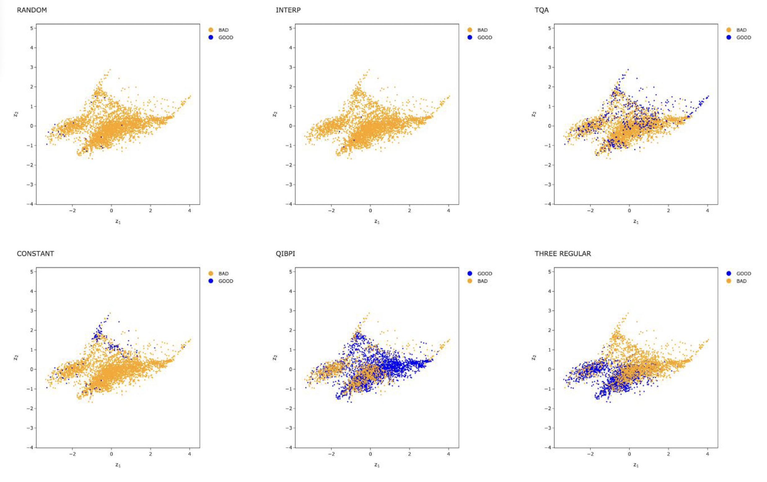
Performance distribution across all initialisation strategies in the instance space.
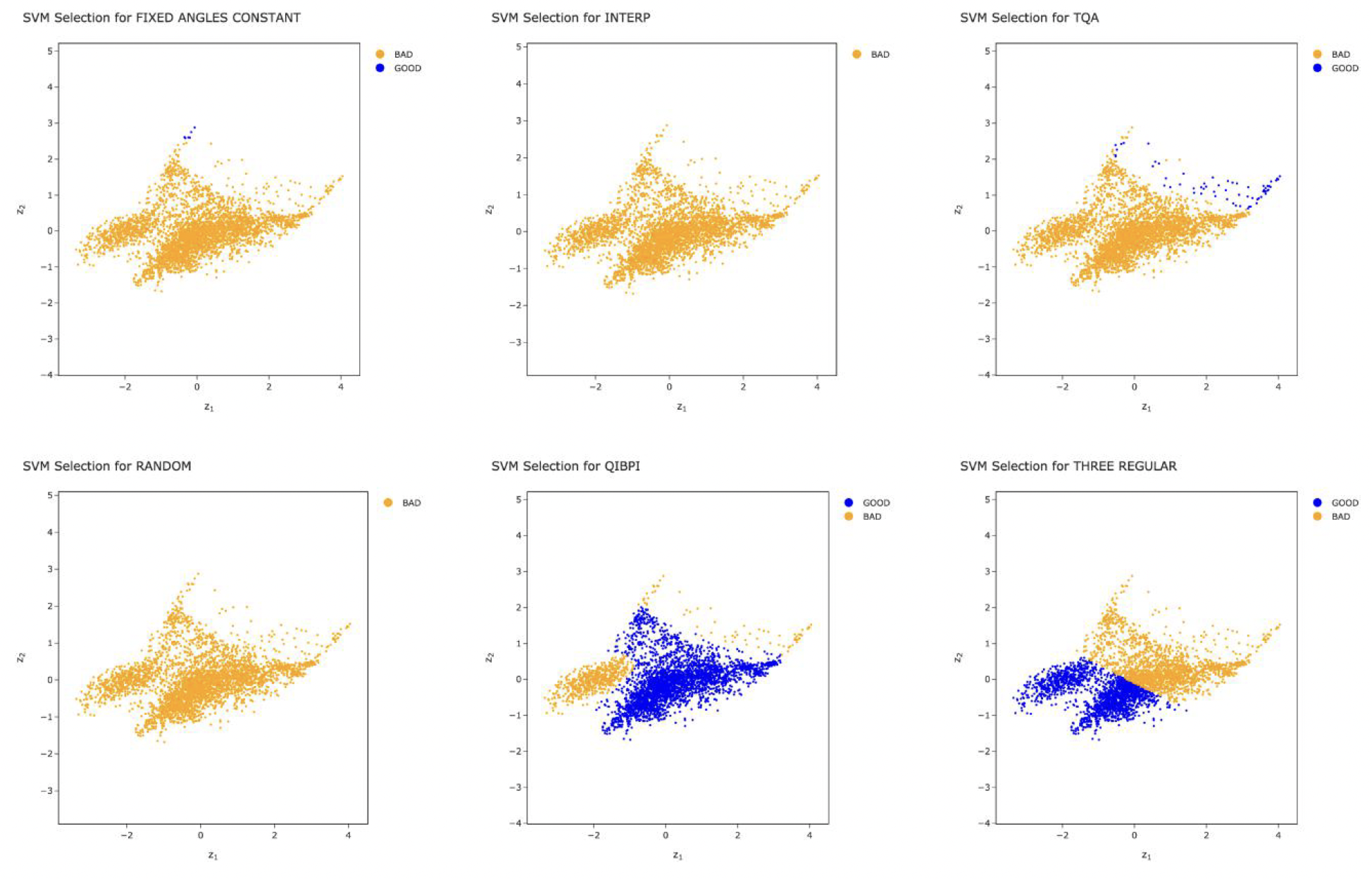
SVM performance boundaries showing where each strategy excels.
The results were striking:
| Strategy | Good instances (%) | CV Accuracy (%) | CV Precision (%) |
|---|---|---|---|
| CONSTANT | 3.2 | 96.7 | 33.3 |
| INTERP | 0.1 | 99.9 | - |
| QIBPI | 70.9 | 75.8 | 78.0 |
| Three-Regular | 44.8 | 78.5 | 73.8 |
| TQA | 11.1 | 90.1 | 87.5 |
| Selector | 77.9 | - | 78.1 |
QIBPI alone achieved 70.9% coverage of "good" instances, and a selector model combining multiple techniques reached 77.9%. The key insight: parameter transfer is effective within instance classes, but not across them.
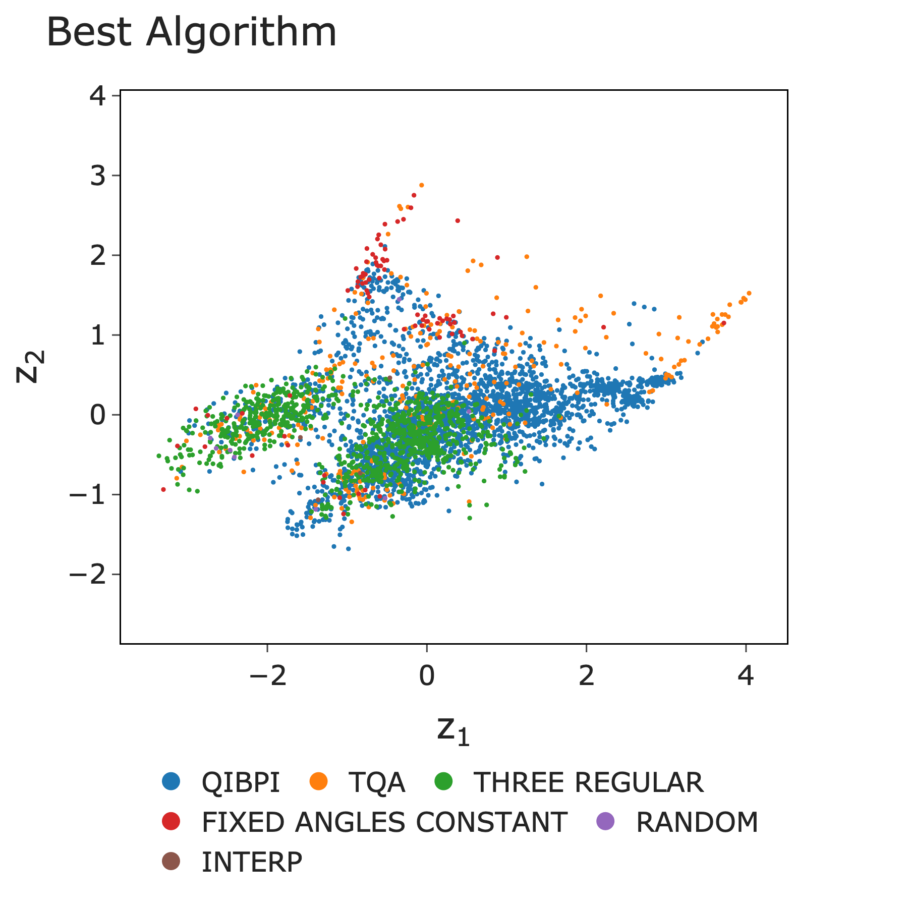
Best algorithm distribution across the instance space.
Evolving Instances to Fill Gaps
Instance Space Analysis revealed gaps, regions of the feature space with no existing instances. To fill these gaps, we used a genetic algorithm approach to evolve new MaxCut instances targeting underrepresented feature regions.
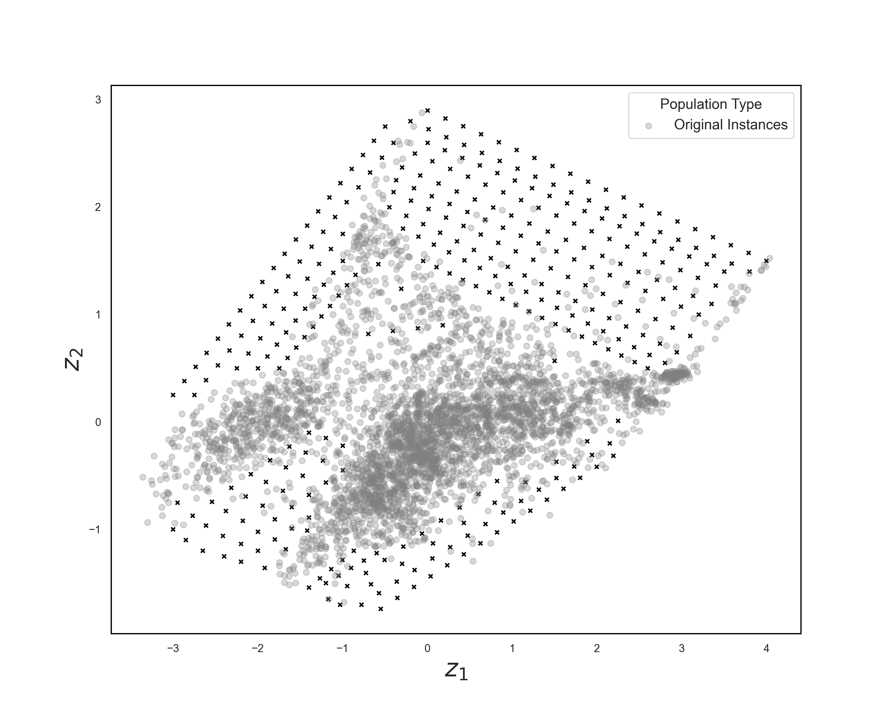
360 target points identified in the instance space for instance evolution.
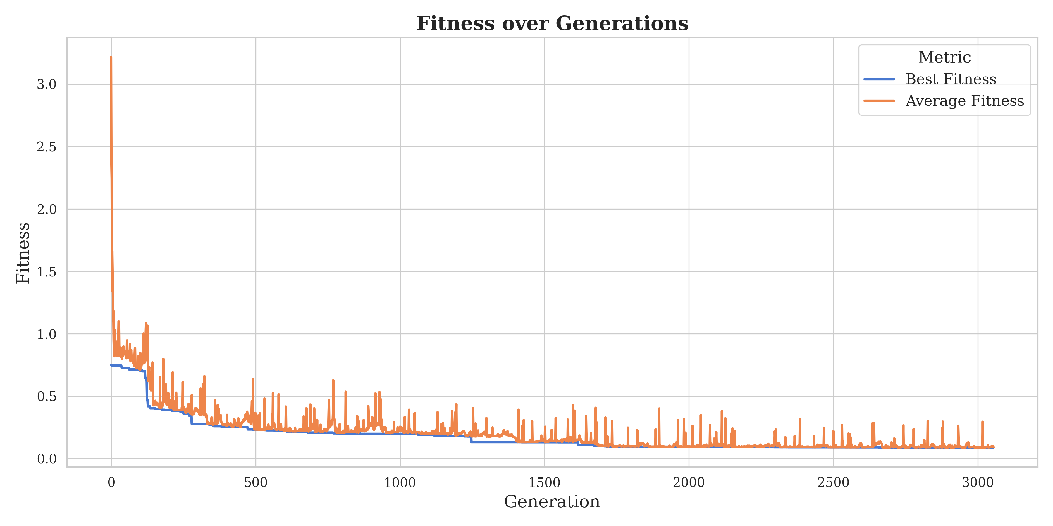
Fitness improvement over generations of the evolutionary algorithm.
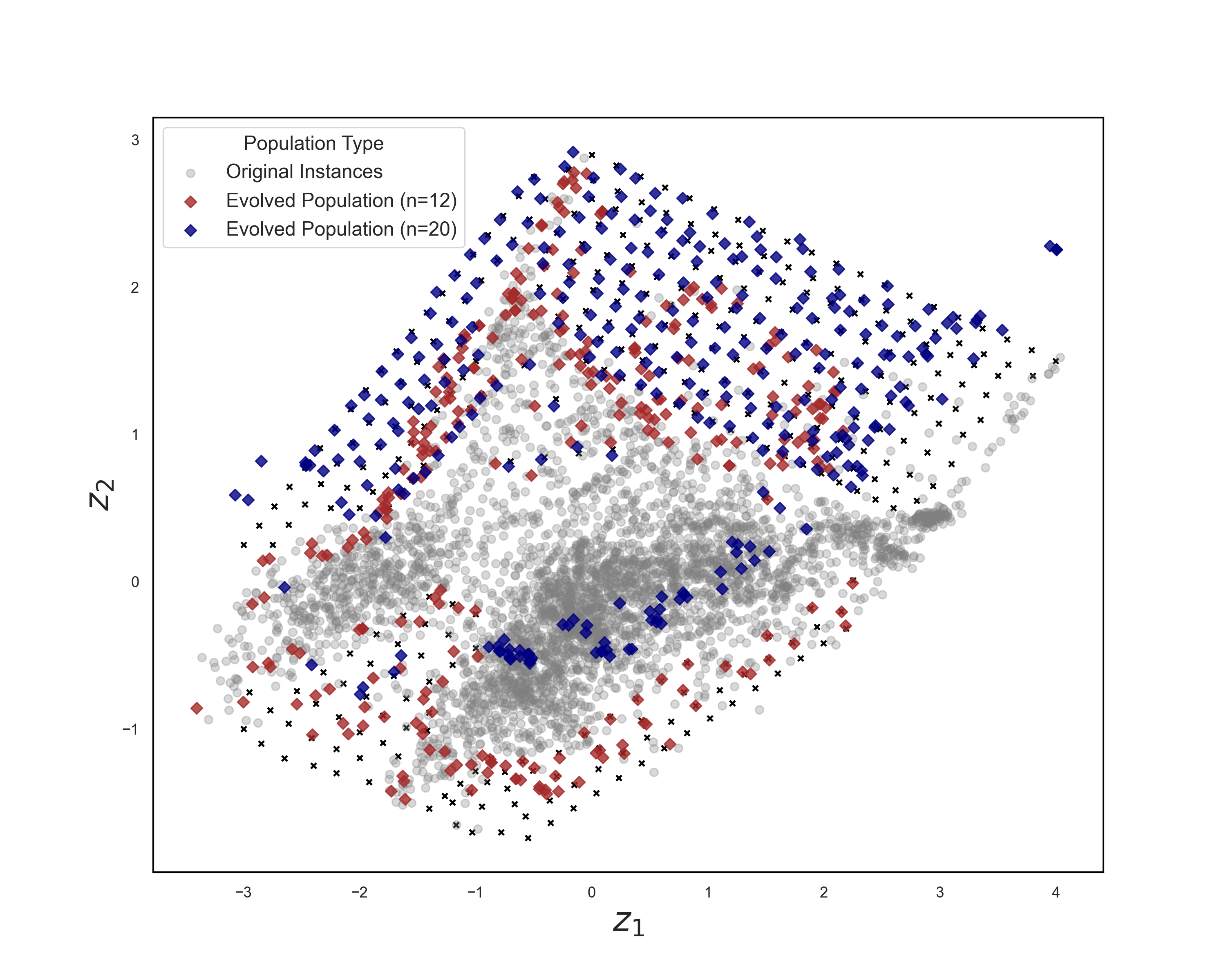
Evolved instances (orange) successfully filling gaps in the original instance space.
Software: QAOA-GamBet
To make these findings practical, we built QAOA-GamBet, a RESTful FastAPI service that consolidates multiple initialisation strategies (Random, QIBPI, QAOAKit, TQA, Constant) into a single, easy-to-use API. It features modular extensibility, built-in validation, and automatic documentation generation.
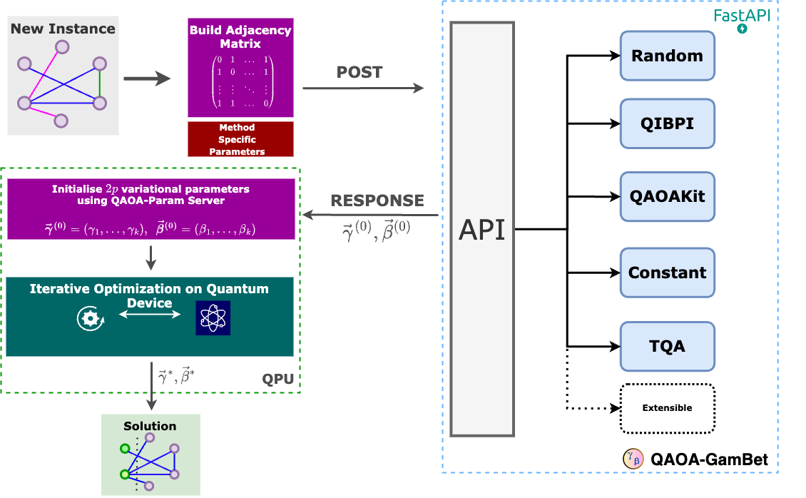
QAOA-GamBet workflow for parameter initialisation.
Key Takeaways
- Instance diversity matters. Testing on narrow instance classes gives a misleading picture of algorithm performance. A diverse test suite of 4,200+ MaxCut instances across 42 classes reveals a much more nuanced story.
- There is no universal best configuration. Instance Space Analysis shows that QAOA design decisions are highly instance-dependent.
- QIBPI works. Our instance-based parameter initialisation strategy achieves 70.9% good instance coverage, and a selector combining multiple techniques reaches 77.9%.
- Parameter transfer works within instance classes, but not across them. This is perhaps the most important finding for practitioners.
- Gaps can be filled. Instance evolution via genetic algorithms generates new instances in underrepresented feature regions, enabling more comprehensive benchmarking.
- QAOA-GamBet makes these findings accessible through a practical API.
This work forms part of Chapters 3 and 4 of my PhD thesis, Instance Space Analysis of Variational Quantum Algorithms. The full thesis is available on Minerva Access.